Project managers: Produce auditable p80 with schedule risk analysis

What does schedule risk analysis actually measure?

Schedule risk analysis answers a narrower question than most people expect. It doesn’t tell you whether your schedule is “good.” It tells you the probability of finishing by a given date, and it separates two very different sources of that uncertainty: the natural variability in how long normal activities take, and discrete risk events that may or may not happen at all.

That distinction matters for how you model the project. A concrete pour taking two extra days because of routine variability is not the same animal as a permit delay that adds sixty days if it materializes, and never happens if it doesn’t. Lump the two together and your simulation blurs the very insight you built it to produce, according to PNNL’s schedule risk analysis guidance, which frames the practice around identifying risks, quantifying their impact on dates and costs, and prioritizing where mitigation actually pays off.

SRA earns its keep at specific moments in a project’s life, not as a one-time exercise filed away after the kickoff meeting:

• Before approval or funding gates, when a sponsor needs a defensible contingency figure rather than a single deterministic date.
• Ahead of major contract milestones, where liquidated damages or bonus clauses hinge on a probability, not a guess.
• At periodic execution checkpoints, typically monthly or tied to major logic changes, to confirm the contingency drawdown still matches actual progress.

Skip any of these windows and the analysis becomes a historical artifact instead of a decision tool.

Preparing a valid CPM schedule and risk register for analysis

A simulation is only as credible as the network feeding it. Garbage logic produces garbage probability curves, no matter how many iterations you run. Before touching a risk tool, work through three preparation steps in order.

1. Clean the schedule. Remove or justify every hard constraint (start-no-earlier-than, must-finish-on), verify that logic ties represent real dependencies rather than leftover placeholders, and confirm calendars reflect actual working days, shifts, and holidays rather than a generic five-day default.
2. Right-size the activity count. Practitioners generally recommend keeping models in the range of roughly 10 to 200 activities unless the underlying plan is unusually mature, since oversized models with thousands of line items routinely fail quality checks and produce three-point estimates nobody can defend, per guidance summarized in the PM World Library’s schedule risk analysis overview.
3. Structure the risk register properly. Fields should separate discrete risks from inherent duration uncertainty, track whether mitigation is already in place or merely planned, assign a clear owner, and define the trigger that forces a review, following the register discipline described in CASRAI’s risk assessment framework.

Skipping this stage is the single most common reason SRA results get challenged during audit or claims review.

The step-by-step method: From estimates to simulation output

Once the schedule and register are clean, the actual analysis follows a repeatable sequence. It isn’t complicated, but skipping a step quietly undermines everything downstream.

Step one: build or summarize the CPM network. Decide activity granularity based on what the analysis needs to answer. A board-level contingency question needs less detail than a claims-defense package. Summary models that collapse detailed contractor schedules into logical work packages are often more reliable than a full, unpruned import, since fewer, better-understood activities beat thousands of poorly estimated ones.

Step two: develop three-point estimates. For each activity (or work package), gather optimistic, most likely, and pessimistic duration values. Where individual estimation is impractical across a large model, apply risk banding: group similar activities into low, medium, and high uncertainty categories rather than forcing unique three-point values everywhere. This preserves consistency and keeps the estimating workload realistic.

Step three: model risks as drivers or discrete events, and link them to activities. This is where AACE’s RP 57R-09 risk-driver method earns its place in the process. A risk driver is a root cause, expressed as a probability of occurrence and a multiplicative impact factor, that can affect multiple activities at once, letting the simulation reflect real correlation rather than treating every duration as independent. A discrete event, by contrast, is a fixed-day hit tied to a specific trigger, such as a permit delay of a defined length. Combining both approaches in a single model is common and often the most realistic way to represent a construction schedule.

Step four: run the Monte Carlo simulation. Choose an iteration count sufficient for stable results. PMI’s guidance on schedule risk analysis points to runs commonly ranging from 500 to 10,000 iterations depending on model complexity and required precision. Rerun at a higher count and compare the resulting P80 date; if it barely shifts, your iteration count is stable. If it swings meaningfully, run more.

Step five: interpret the outputs. You’ll get a probability distribution of finish dates, key percentile markers such as P50, P80, and P90, and a tornado or sensitivity chart ranking which activities or risk drivers contribute most to schedule variability.

• P50 represents a coin-flip date: half of simulated outcomes finish earlier, half later.
• P80 or P90 are the levels most organizations use for contingency planning, since they reflect a higher confidence threshold than the deterministic finish date most schedules report.
• The tornado chart tells you where mitigation dollars produce the most schedule benefit, which is often not the activity sitting on the original critical path.

Pro Tip: Run the simulation twice at different iteration counts before trusting the P80 figure in a board presentation. If the two runs land within a day or two of each other, the model has converged. If they don’t, the instability usually traces back to too few iterations or a risk driver with an unrealistically wide impact range.

Model quality checklist and technical considerations

A statistically sound Monte Carlo run can still produce a misleading answer if the underlying model has structural flaws. Before presenting results, run through a short quality checklist grounded in AACE’s RP 64R-11 recommended practice:

• No forcing constraints remain in the schedule that would artificially cap or float a date regardless of simulated duration.
• Calendars match actual working patterns across all linked activities, including subcontractor-specific work weeks.
• Logic ties are valid, meaning no dangling activities, no unjustified lags, and no circular references.
• Every material assumption behind the three-point estimates is disclosed, not buried in a spreadsheet nobody reviews.

Two technical effects deserve particular attention. Merge bias occurs where multiple parallel paths converge on a single successor activity. Because the successor can’t start until every predecessor finishes, the simulated finish date skews later than intuition suggests, and this effect grows sharply as the number of converging paths increases. Correlation between activity durations matters whenever the same crew, weather exposure, or supplier drives multiple tasks; ignoring it tends to understate the true spread of outcomes, while a risk-driver structure that ties one root cause to several activities is the practical way to test and represent it.

Choosing between a summary model and a fully detailed one comes down to what decision the analysis supports. A funding-approval question rarely needs contractor-level granularity, and a bloated model often makes quality control harder, not more precise.

Common pitfalls and best practices

Certain mistakes show up in schedule risk analysis often enough to name specifically. Watch for these:

• Using PERT instead of Monte Carlo on a real CPM network. PERT tends to understate risk on any project with parallel paths, because it doesn’t account for merge bias, and PMI’s guidance on simulation warns that PERT can produce a false sense of confidence on exactly the projects where risk analysis matters most.
• Importing a contractor’s full detailed schedule without pruning it. Thousands of unreviewed activities do not make a model more accurate. They make it slower to run and harder to audit, and they dilute attention away from the handful of activities that actually drive the finish date.
• Assigning false precision to a risk register. A “72% probability, 14-day impact” entry sounds rigorous but is rarely defensible when the underlying data is a project manager’s gut estimate. Ordinal banding (low, medium, high) preserves consistency without pretending to a precision the inputs don’t support.

Pro Tip: Set review triggers around events, not calendar dates alone, such as “reopen this risk when the permit application is submitted” rather than “review quarterly.” Event-based triggers keep the register tied to what’s actually happening on site instead of turning into a stale compliance form.

Software tools and the data that feeds them

Tool selection matters less than most vendors imply, but a few capabilities are non-negotiable for credible schedule risk analysis. Look for CPM-compatible simulation that reads your native schedule format without manual re-entry, native support for risk-driver linkage rather than treating every activity as independently uncertain, built-in distribution templates for common duration shapes, correlation modeling, and clear sensitivity or tornado chart output.

Iteration settings deserve a deliberate test rather than a default. Run the simulation at, say, 1,000 iterations, note the P80 date, then rerun at 10,000 and compare. Convergence within a day or two confirms the lower count was adequate for that model; a bigger gap means the risk drivers or activity count are pushing the model toward instability.

Data hygiene behind the three-point estimates matters as much as the tool itself. Historical productivity records, subcontractor input, and prior project closeout data all beat guesswork for duration ranges. Where weather or seasonal access genuinely affects a schedule, probabilistic calendars that reflect historical weather-day loss rates produce far more defensible results than a flat assumption of “good weather” baked into the base schedule.

How an AI civil-engineer workflow speeds SRA preparation

Most of the time spent on schedule risk analysis isn’t spent running the simulation. It’s spent cleaning the schedule, chasing down evidence for three-point estimates, and reconciling a risk register that hasn’t been touched since the last audit. This is where an AI civil engineer like Yesper changes the workload rather than the method.

• Yesper can flag broken logic, unjustified constraints, and calendar mismatches across a large CPM file faster than a manual review pass.
• It can extract candidate risk drivers and supporting evidence from project documents, correspondence, and prior closeout reports for an analyst to validate.
• It can surface a first draft of three-point ranges based on comparable historical activities, which a risk analyst then checks, adjusts, and signs off on.

The output is always a suggestion, never a final answer. Human-in-the-loop verification, where the analyst reviews and records every assumption the way they would review a colleague’s work, stays central to a defensible SRA package. For a broader look at how this kind of workflow fits into engineering practice, see what an AI civil engineer actually does.

Turning probability distributions into contingency decisions

The simulation output is only useful once it changes a decision. Start by picking a confidence level consistent with your organization’s risk appetite. A publicly funded infrastructure program with heavy political scrutiny might target P90 for schedule contingency, accepting a wider buffer to avoid a public overrun. A fast-moving private developer with higher risk tolerance might set contingency at P70 or P80 instead.

• Convert the chosen percentile into a time-based contingency by comparing it against the deterministic (unrisked) finish date; the gap is your buffer.
• Establish a drawdown procedure that releases contingency as risks are retired or pass their trigger window without occurring, rather than holding the full buffer until the final month.
• Use the sensitivity ranking to direct mitigation budget toward the top three or four drivers, not the activity that happens to sit on the nominal critical path.

Rerun the analysis whenever a major driver is resolved, a significant logic change hits the schedule, or a milestone approaches. A distribution built at project kickoff has limited value eighteen months into execution.

Beyond monte carlo: Other schedule risk methodologies

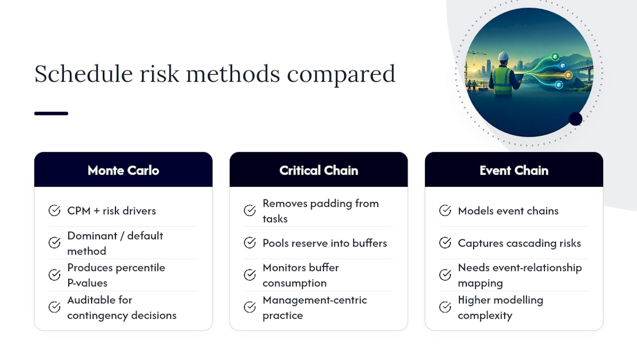
Monte Carlo simulation on a CPM network is the dominant method, but it isn’t the only one, and understanding the alternatives clarifies why Monte Carlo remains the default for most quantitative work.

Critical Chain Project Management approaches schedule risk differently by removing padding from individual task estimates and pooling that reserve into project and feeding buffers placed strategically in the network. Rather than asking “what’s the probability of finishing by date X,” Critical Chain asks “how much buffer consumption signals a real threat to the project buffer.” It’s a management method as much as an analytical one, and it works best on organizations willing to change how individual task owners estimate and report progress. It doesn’t produce the same P-value distributions that Monte Carlo does, which makes it harder to translate into the percentile-based contingency conversations that funders and sponsors expect.

Event Chain Methodology extends CPM by modeling chains of events, where one risk event increases the probability or severity of a subsequent event, rather than treating each risk as isolated. It’s particularly suited to projects where risks cascade, a permitting delay that increases the probability of a subsequent weather-window miss, for example. Event Chain requires more sophisticated event-relationship mapping than standard Monte Carlo and is used less broadly in construction, largely because the extra modeling complexity often isn’t justified unless the project has clearly interdependent risk chains.

For most construction and infrastructure work, Monte Carlo on a well-prepared CPM network with risk drivers, as recommended by AACE and PMI, delivers the clearest, most auditable results for contingency and approval decisions. The other methods are worth knowing, but they solve narrower problems.

Making SRA part of project governance, not a one-off report

Schedule risk analysis loses most of its value when it’s treated as a document produced once and filed; its real function is feeding decisions: gate approvals, contract negotiations, contingency drawdown, and monthly progress reviews all depend on a current probability picture, not the one calculated at kickoff.

That means SRA needs to sit inside your existing project controls cadence rather than beside it. Whoever owns the monthly schedule update should also own triggering a rerun when logic changes materially, when a top-ranked risk driver resolves or worsens, or when a milestone approval is coming up. Treat the risk register the same way; a register nobody has touched in six months is not a risk register, it’s an archive.

Practically, this works best with clear ownership. A single risk analyst or scheduler should hold responsibility for maintaining the model and register between formal SRA runs, with a project controls manager or sponsor signing off on any change to the confidence level used for contingency. Reviews tied to events, a permit decision, a major subcontract award, a design freeze, keep the analysis relevant without turning it into a bureaucratic monthly checkbox.

Explaining results to non-technical stakeholders

A P80 finish date and a tornado chart mean nothing to a sponsor who thinks in terms of “will we hit the date or not.” Translating probabilistic output into language that supports a real decision is a skill separate from running the simulation itself.

Lead with the decision the number supports, not the statistical mechanics behind it.

Visuals do more work than tables here. A cumulative probability curve showing the S-curve of finish dates, with the deterministic date, P50, and P80 marked clearly, communicates the spread in seconds. A tornado chart ranking the top five risk drivers by schedule impact tells a sponsor exactly where their attention and mitigation budget should go, which is usually more persuasive than any narrative description.

Avoid overloading a steering committee with the full model. Reserve activity-level detail for the working session with the scheduler and risk analyst, and bring only the finish-date distribution, the recommended contingency, and the top driver list to the decision-making audience. Reruns and updates should be flagged the same way, with a short note on what changed and why the recommended contingency moved, rather than a full re-presentation of the entire analysis each time.

Building schedule risk analysis into everyday controls

SRA delivers the most value when it stops being a special-occasion report and becomes a routine input to how a project is governed. That means tying reruns to real triggers, not an arbitrary calendar, and keeping the risk register alive through active ownership rather than a one-time entry at kickoff.

Ownership should be explicit: a named scheduler or risk analyst maintains the model between formal runs, and a controls manager or sponsor signs off whenever the confidence level driving contingency changes. Reviews tied to permits, design freezes, or major subcontract awards keep the whole exercise honest.

How Yesper supports schedule risk analysis work

Building a credible schedule risk model still takes real analytical judgment, but the preparation work around it, cleaning a CPM file, tracing evidence for three-point estimates, and keeping a risk register current, is exactly the kind of document-heavy task an AI civil engineer like Yesper is built for. Yesper can scan a schedule for broken logic and constraint issues, pull risk-driver evidence out of correspondence and prior project records, and surface draft duration ranges for an analyst to review and adjust, all while showing its assumptions so a risk analyst can check them the way they’d check a colleague’s work. It is used across teams at construction and engineering firms for exactly this kind of document-heavy, judgment-critical work. If your team is spending more time reconciling schedules than actually analyzing risk, it’s worth seeing how that preparation work could be handled differently. Learn more about Yesper’s platform and services or read how one engineering firm approaches searchable project knowledge in the COWI case study.

Selected primary sources and recommended reading

For readers who want the underlying recommended practices rather than a summary, these are the sources practitioners cite most:

• AACE RP 64R-11 covers CPM schedule quality requirements and model-building choices in full technical detail.
• AACE RP 57R-09 explains the risk-driver method for integrated cost and schedule analysis.
• PMI’s schedule risk analysis guidance offers a practitioner-level walkthrough of Monte Carlo simulation on CPM networks.
• PNNL’s schedule risk analysis overview frames the core questions SRA is meant to answer.
• NIST’s AI Risk Management Framework is a useful crosswalk where AI tools support risk-register governance.